K-mer analysis and genome size estimate

Genome size can be calculated by counting k-mer frequency of the read data. The k should be sufficiently large that most of the genome can be distinguished. For most eukaryotic genomes at least 17 are usually used and calculation upto 31 is easiliy doable with Jellyfish.

Prerequisite

Here we assume the following are available.

• Jellyfish
• R
• large volume of raw read data with quality(fastq)

Outline

1. count k-mer occurence using Jellyfish (jellyfish count)
2. summarize as histogram (jellyfish histo)
3. plot graph with R
4. determine the total number of k-mer analyzed and the peak position
5. compare the peak shape with poisson distribution

Count k-mer occurence

In this example we have 5 pair of fastq files in three different subdirectories. The file to process can be specified with "*/*.qf.fastq" and veriied with ls.

$ ls */*.qf.fastq
run1/s_1_1_sequence.qf.fastq  run2/s_2_2_sequence.qf.fastq
run1/s_1_2_sequence.qf.fastq  run3/s_1_1_sequence.qf.fastq
run2/s_1_1_sequence.qf.fastq  run3/s_1_2_sequence.qf.fastq
run2/s_1_2_sequence.qf.fastq  run3/s_2_1_sequence.qf.fastq
run2/s_2_1_sequence.qf.fastq  run3/s_2_2_sequence.qf.fastq

Next, we issue the jellyfish count command

jellyfish count -t 8 -C -m 25 -s 5G -o spec1_25mer --min-quality=20 --quality-start=33 */*.qf.fastq

-t 8

specifies the number of threads to be used. This value should be equal to the number of cores on the machine or the number of slots you reserved through job management system ($NSLOTS in SGE or UGE).

-C

specifies the both strands are considered. If you do not specify this, the apparent depth would be half, --- that is undesirable

-m 25

specified that now you are counting for 25 mer (i.e., k=25)

-s 5G

is some kind of magical number specification of hash size. This should be as high as the physical memory allows. The higher the faster, but exceeding the available memory leads to failure or extremely slow counting.

-o spec1_25mer

specifies the prefix of output file names.

--quality-start=33

specified that your fastq file have 33 based quality value string. Be careful on the dataformat. There are cases that your data are 64 based depending on the sequending system and software versions. This is relevant only when you specify --min-quality

--min-quality=20

specifies that nucleotide having qv lower than 20 should not included in the count. This selection reduces the k-mers derived from sequence errors and make the peak clearer.

*/*.qf.fastq

will be expanded to the ten filenames explained above by the shell and passed to jellyfish as input files

summarize as histogram (jellyfish histo)

First confirm that you got the output file

$ ls spec1_25mer*
spec1_25mer_0

now that there is a single file spec1_25mer_0

$ jellyfish histo -o spec1_25mer.histo spec1_25mer_0

Confirm that you got the output

$ ls spec1_25mer*
spec1_25mer_0  spec1_25mer.histo

Examine the numbers by your eyes

$ head -25 spec1_25mer.histo
1 461938583
2 95606044
3 19280477
4 13836754
5 11018480
6 9555090
7 8557935
8 7863244
9 7319505
10 6920880
11 6589723
12 6321923
13 6148638
14 6036120
15 5972264
16 5962234
17 5987696
18 6051171
19 6154429
20 6297373
21 6485135
22 6700579
23 6932570
24 7217627
25 7533211

Plot graph with R

$ R
...
> spec1_25 <- read.table("spec1_25mer.histo")
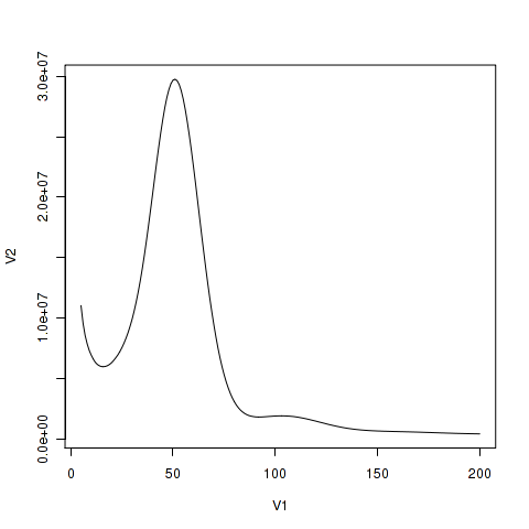
> plot(spec1_25[5:200,],type="l")

This will plot from 5 th line in the histo file. In general, the very low frequency k-mer are extremely high number that would make the scale for the y-axis too large. For x values, selection of the higher bound should be determined in accordance with read depth. The data contains upto 10000. However if you plot them, it would be too large. Thus some good number should be chosen.

Determine the total number of k-mer analyzed and the peak position

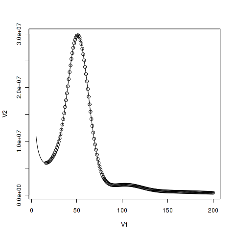
First, you should determine the border between the peak corresponding to single copy region and the initial peak corresponding to sequence errors. You might plot points on the line so that the region would be obvious.

> points(spec1_25[16:200,])

Now, we would calculate the total number of k-mer in the distribution

> sum(as.numeric(spec1_25[16:10000,1]*spec1_25[16:10000,2]))
[1] 120107242393

In this case there are about 120 G k-mers in the histogram.

Next, we want to know the peak position. From the graph, we can see its close to 50. Thus we examine the number close to 50 and find the maximum value

spec1_25[40:60,]
   V1       V2
40 40 20225459
41 41 21557020
42 42 22881520
43 43 24132924
44 44 25331980
45 45 26419451
46 46 27411481
47 47 28246677
48 48 28903809
49 49 29388497
50 50 29680473
51 51 29751275
52 52 29636175
53 53 29324357
54 54 28809699
55 55 28107532
56 56 27232397
57 57 26208735
58 58 25075370
59 59 23840233
60 60 22522009

In this example, the peak is at 51. Then, the genome size can be estimated as:

> sum(as.numeric(spec1_25[16:10000,1]*spec1_25[16:10000,2]))/51
[1] 2355043968

This reads as 2.36 Gb.

If we regard single copy region as frequency between 16 and 80, the size of single copy region can be roughly calculated as

> sum(as.numeric(spec1_25[16:80,1]*spec1_25[16:80,2]))/51
[1] 954755030

It is 0.95 Gb or 40.5% of the genome. The proportion could be calculated as:

> (sum(as.numeric(spec1_25[16:80,1]*spec1_25[16:80,2]))/sum(as.numeric(spec1_25[16:10000,1]*spec1_25[16:10000,2]))
[1] 0.4054086

For an inbred line, two set of genomes have mostly identical sequence and the major peak would be diploid (2C) peak. On the otherhand, for highly heterozygous sample, there would be heterozygous peak with 1C depth.

compare the peak shape with poisson distribution

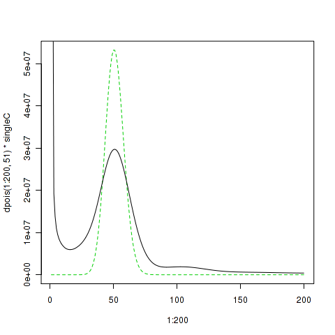
Now that we have some nice curve, we could compare it to ideal curve as poisson distribution scaled to the estimated single copy region size

> singleC <- sum(as.numeric(spec1_25[16:80,1]*spec1_25[16:80,2]))/51
> plot(1:200,dpois(1:200, 51)*singleC, type = "l", col=3, lty=2)
> lines(spec1_25[1:200,],type="l")